Alpine Sentiment Analysis

This article includes the following sections:

• Introduction to Sentiment Analysis
• Example Data
• GPText Analysis
• Alpine Data Transformation
• Alpine Sentiment Model
• Conclusion

Introduction to Sentiment Analysis

If social websites such as Twitter and Facebook have taught us anything, it’s that people are not afraid to express their opinions openly on public forums. While most opinionated posts on the internet reach a very small audience of friends and families, some people have developed large social followings which give their words weight. An audience of millions reads anxiously when LeBron James tweets about his preference for basketball shoes. The opinions being expressed about brands is valuable information that allows companies to tweak their products and marketing campaigns in order to find and retain customers. As the volume of data being created on social websites continues to grow it has become impossible for companies to react to trending opinions without the aid of automated sentiment analysis.

Although sentiment analysis has become more popular in recent years, it has yet to become an easy problem to solve. Text must be cleansed, parsed, and analyzed before a statistical model can be developed that is capable of automatically determining whether the writer was expressing a positive or negative opinion about a particular brand. The complexity of these tasks has proved daunting to most companies, but this article describes an approach for using Alpine, Greenplum, and GPText to easily create a sentiment analysis model.

Example Data

The data used in the following examples are user created movie reviews from the website Rotten Tomatoes. This data was originally collected for a paper published by Bo Pang and Lillian Lee. A sentiment score was determined as follows:

We assumed snippets (from Rotten Tomatoes webpages) for reviews marked with
``fresh'' are positive, and those for reviews marked with ``rotten'' are
negative.

An example of a positive review is:

offers that rare combination of entertainment and education 

A negative review might look like:

it's so laddish and juvenile , only teenage boys could possibly find it funny

Our goal is to use these reviews which have a known sentiment score to create a machine learning model capable of predicting the sentiment of unlabeled reviews.

GPText Analysis

Before any text analytics are possible we must first transform our text documents into data structures that we can apply mathematical models to. This data structure is known as a Term Vector. A naive approach to creating a term vector might be to split a document on white space and put each resulting term into an array. In practice we will see much better results by applying a more sophisticated Analyzer Chain that removes punctuation and stop words, checks for synonyms, stems words into root terms, etc. Many libraries exist that are capable of turning documents into term vectors, but for this example we will use GPText.

GPText is an add-on package for the popular Greenplum database that brings text analytics capabilities to the parallel platform. It uses the industry standard Lucene and Solr libraries for analyzing and indexing text. All of the functionality is exposed through SQL and can be combined with all the other features of the database engine.

First we load our demo data set into a Greenplum table. The only three fields we need to store are an identifier, the message itself, and polarity to indicate whether the review was positive or negative.

id   |                                     message                                      | polarity
------+----------------------------------------------------------------------------------+---------+
7    | offers that rare combination of entertainment and education .                    | pos
5333 | it's so laddish and juvenile , only teenage boys could possibly find it funny .  | neg

Next we create a GPText index on our table using the create_index() database function.

demo=> SELECT * FROM gptext.create_index( 'public', 'review', 'id', 'message' );
INFO:  Created index demo.public.review
create__index
--------------
t
(1 row)

Since we will want to do more than just search our documents we also need to enable extracting term vectors from the message field.

demo=> SELECT * FROM gptext.enable_terms( 'demo.public.review', 'message' );
INFO:  Successfully enabled term support on field message in index demo.public.review.  A reindex of the data is required.
enable_terms
--------------
t
(1 row)

Now we simply index our data and commit the transaction.

demo=> SELECT * FROM gptext.index( TABLE( SELECT * FROM review ), 'demo.public.review' );
demo=> SELECT * FROM gptext.commit_index( 'demo.public.review' );
commit_index
--------------
t
(1 row)

Even though it isn’t our primary goal, we can now search our documents inside the database using a fully featured search engine instead of just regular expressions.

demo=> SELECT q.id, q.score, r.message, r.polarity FROM gptext.search( TABLE( SELECT 1 SCATTER BY 1 ), 'demo.public.review', 'laddish AND possibly', null ) q, review r WHERE q.id = r.id;
id   |       score       |                                     message                                      | polarity
------+-------------------+----------------------------------------------------------------------------------+
5333 | 0.353553384542465 | it's so laddish and juvenile , only teenage boys could possibly find it funny .  | neg
(1 row)

Finally we can exercise arguably the most powerful feature of GPText, which is extracting the term vectors from the text search engine into a database table.

demo=> CREATE TABLE myterms AS SELECT * FROM gptext.terms( TABLE( SELECT 1 SCATTER BY 1 ), 'demo.public.review', 'message', '*:*', NULL );
SELECT 16

We now have a table which contains the analyzed terms and their positions in every document of our corpus

demo=> SELECT * FROM myterms WHERE id=7;
id |   term    | positions
----+-----------+-----------+
7  | combin    | {3}
7  | educ      | {7}
7  | entertain | {5}
7  | offer     | {0}
7  | rare      | {2}
(5 rows)

We will use this table as the base for all analytics to follow. The first useful thing we can do with our terms table is to create a dictionary for our corpus:

CREATE TABLE dictionary AS
    SELECT
        row_number() OVER( ORDER BY term ASC ) dic,
        term,
        count(*) AS count
    FROM review_terms WHERE term IS NOT NULL GROUP BY term DISTRIBUTED RANDOMLY;

Alpine Data Transformation

Now that we have a table in our database which contains the term vectors for each document, we can start working with Alpine to build a Sentiment Analysis model. We will create two Alpine workflows: the first will be a transformation flow and the second will be our predictive model.

Our first Alpine workflow takes the original review table, the term vector table, and our dictionary table and combines them into a single table we use with our predictive model.

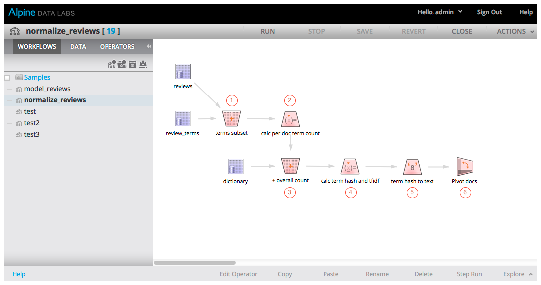
The steps in the above workflow are described as follows:

1. We first use the Join operator to combine the review table with the term vector table
2. Calculate the number of times each distinct term appears in each document using the Variable operator
3. Join to our dictionary table to find the number of times each distinct term appears in the overall corpus
4. Use the Variable operator to calculate two new fields:
   1. Calculate the TF-IDF score for each term of each document. This will allow us to measure how important each word is and give us a much more accurate model.
   2. Use the feature hashing trick to reduce the dimensionality of each document’s feature vector. This will allow us to control the size of our feature vectors, without it the size of each feature vector would be equal to the number of terms in the corpus dictionary
5. Transform the term hash we just calculated into a string using the Numeric to Text operator so we can use it as a categorical variable in later steps
6. We now have a table with one row for each unique term of each document in our corpus. The last step of this flow is to Pivot that table so we have one row per document containing one column per term

An example row from our final output table looks like the following. It contains one row for each document. That row contains the id of the review and one column per term. If the term doesn’t exist in the document then the value will be 0; if it does exist, then the value will be the tf-idf score, which indicates the importance, or weight, of that term in that particular document.

demo=> SELECT * FROM review_term_pivot LIMIT 1;
 id | term_hash_99  | term_hash_98 |   term_hash_97   |  . . .   |  term_hash_1
  1 |             0 |            0 | 2.81756536955978 |  . . .   |  1.4623979 

Alpine Sentiment Model

We can use the output from our transformation flow to build a predictive model. There are many different methods available for building a sentiment analysis model. The effectiveness of each approach will depend largely on the data set being analyzed, so it is up to each data scientist to discover a method that works for them. For our simple example we will build a Naive Bayes model.

The steps in the above workflow are described as follows:

1. Remember that the polarity for each document in our original data set was represented as the strings ‘positive’ or ‘negative’, we first use the Variable operator to transform that value into a 1 for positive or a 0 for negative
2. Next we Join the transformed polarity value to the pivot table created in the above transformation workflow
3. Use the Random Sample operator to split our data into a Training Set and Validation Set. For this example we directed 80% of the data into the training set and 20% to the validation set
4. The Naive Bayes operator is used to build our predictive model. Polarity is set as our dependent variable and each of our 200 term columns are used as predictors.
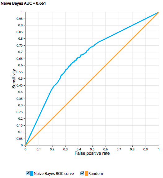
5. Use the Naive Bayes model and our validation data set to create a ROC curve to measure the performance of our model
6. Create an output table using the Predictor operator which will append prediction and confidence columns to our reviews

The output of the ROC operator shows us that this model received an AUC score of 0.661. This means there is roughly a 66% probability we will rank a randomly chosen positive review higher than a randomly chosen negative review. This may not be a high enough probability for many applications, but it does show us this model has promise. We could spend time tweaking the inputs or add additional data to improve our sentiment analysis model.

Finally we can examine our resulting prediction table to see the actual polarity, our predicted polarity, and the confidence scores for each movie review in our validation data set.

demo=> SELECT id, positive, "P(positive)", "C(1)", "C(0)" FROM review_predictions LIMIT 10;
id  | positive | P(positive) |         C(1)         |         C(0)
------+----------+-------------+----------------------+----------------------+
3097 |        1 |           0 |    0.349999267862347 |    0.650000732137653
1848 |        1 |           0 |    0.135203052587874 |    0.864796947412126
3141 |        1 |           1 |    0.934236014015589 |   0.0657639859844111
5155 |        1 |           0 | 4.55551627779962e-06 |    0.999995444483722
9962 |        0 |           1 |    0.999833818119476 | 0.000166181880523784
6933 |        0 |           0 | 1.01096047849114e-06 |    0.999998989039522
4652 |        1 |           0 |  1.9685909226364e-06 |    0.999998031409077
4491 |        1 |           1 |      0.9915488901559 |  0.00845110984410007
5621 |        0 |           0 | 2.04184094342355e-07 |    0.999999795815906
3466 |        1 |           1 |    0.957841355771335 |   0.0421586442286655
(10 rows)

Conclusion

We’ve seen a simple approach to using Alpine and GPText to build a Sentiment Analysis model. Our final model isn’t as predictive as one might like, but there is clearly ample room for improvement. Using Alpine, only one operator would need to be replaced to switch from Naive Bayes to a Support Vector Machine, which may arguably be more predictive for this use case. One could imagine the final model being used to score the sentiment of human generated content as it is produced with the result being visualized in a user facing application. For example, a brand manager could have access to a graph which depicts the real time Twitter response to a new marketing campaign.